Decision Tree in R

Decision Trees are non-parametric supervised learning method that are often used for classification and regression. The basis of decision trees is to create simple rules to decide the final outcome based on the available data. It uses a visualization or graphical method to explain the rules and take the final decision.

Advantages of decision trees:

• Simple to understand and to interpret. Trees can be visualized.
• Requires little data preparation.
• Able to handle both numerical and categorical data
• Useful in data exploration
• Non-parametric method, thus it does not need any assumptions on the sample space

Disadvantages:

• Over fitting and unstable at times
• Loses a lot of information while trying to categorize continuous variable
• Not sensitive to skewed distribution

A few terminologies related to decision tree are as follows:

1. Root Node: The starting point of a tree which captures the entire data.
2. Splitting: Process of diving a node into two or more sub-nodes.
3. Decision Node: When a sub-node splits into further sub-nodes, then it is called decision node.
4. Leaf or Terminal Node: Nodes that are not split any further are called as terminal node or leaf.
5. Pruning: Stopping a node to split into further sub-nodes.
6. Branch or Sub-Tree: A sub section of entire tree is called branch or sub-tree
7. Parent and Child Node: A node, which is divided into sub-nodes is called parent node of sub-nodes whereas sub-nodes are the child of parent node.

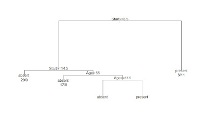
Next we will run a decision tree in R, and look into the lot. We will use the RPART package in R for this. RPART comes with a number of in-built datasets, and we will use the dataset named “kyphosis” for our project.

# RPART is the package for running decision tree

install.packages("rpart")

library(rpart)

# This is an in-built dataset in the RPART package

kyphosis

# The basic code for implementing a Decision Tree

fit1 <- rpart(Kyphosis ~ Age + Number + Start, data = kyphosis)

# These will plot the tree

plot(fit1)

text(fit1, use.n = TRUE)

# A more fancy plot can be obtained using the following packages. This is optional.

install.packages("rattle")

install.packages("rpart.plot")

install.packages("RColorBrewer")

library(rattle)

library(rpart.plot)

library(RColorBrewer)

fancyRpartPlot(fit1)

# Code to predict and score dataset using the decision tree created above.

# In this case, we are trying to do an in-sample validation

pred1 <- as.data.frame(predict(fit1,kyphosis))

# Creating a final table and assigning 1 where predicted probability is greater than 1

pred_kyphosis1 <- data.frame(act_kyphosis = kyphosis$Kyphosis, prob = pred1$present)

pred_kyphosis1$prediction[pred_kyphosis1$prob >= 0.5] = "Pred_Present"

pred_kyphosis1$prediction[pred_kyphosis1$prob < 0.5] = "Pred_Absent"

# Creating the classification (or confusion matrix)

prop.table(table(pred_kyphosis1$act_kyphosis,pred_kyphosis1$prediction))

	Pred_Absent	Pred_Present
Absent	0.65	0.14
Present	0.02	0.19

There are multiple options available while running a decision tree. Here, we will explore one such example of using a loss function.

Suppose, in our case the precision rate should be high, while we can allow the recall rate to go down a bit. Therefore, we want our predictions to be more accurate, i.e. we want our FALSE POSITIVE to be low, even though it may lead to cases where actual 1's are not getting captured, therefore the FALSE NEGATIVE going up.

We can include the cost function in the code where we build the decision tree.

# Creating a Decision Tree with loss function

fit2 <- rpart(Kyphosis ~ Age + Number + Start, data = kyphosis,

              parms=list(split="information", loss=matrix(c(0,2,1,0), byrow=TRUE, nrow=2)))

pred2 <- as.data.frame(predict(fit2,kyphosis))

pred_kyphosis2 <- data.frame(act_kyphosis = kyphosis$Kyphosis, prob = pred2$present)

pred_kyphosis2$prediction[pred_kyphosis2$prob >= 0.5] = "Pred_Present"

pred_kyphosis2$prediction[pred_kyphosis2$prob < 0.5] = "Pred_Absent"

# Classification matrix for the new tree

prop.table(table(pred_kyphosis2$act_kyphosis,pred_kyphosis2$prediction))

	Pred_Absent	Pred_Present
Absent	0.74	0.05
Present	0.10	0.11

We can clearly see how the FALSE POSITIVE has gone down, and FALSE NEGATIVE has increased.